
Carbdown Fluxmeter Army: Building Robotic Scientific Instruments For CO₂ Efflux Monitoring Of EW Experiments
Why and how we built our army of autonomous CO₂ fluxmeters
Blog article - V1.0 - Feb 8th 2024 - Dirk Paessler, Ralf Steffens, Jens Hammes, Anna Stöckel, Ingrid Smet

Introduction

Enhanced weathering (EW) is expected to become one of the keystones to fight climate change by capturing CO₂ from the atmosphere and storing it underground and in the oceans at reasonable cost. However, as the exact inner workings of the involved processes are not yet fully understood, a lot more scientific data is needed for the ongoing development of this carbon dioxide removal (CDR) method.
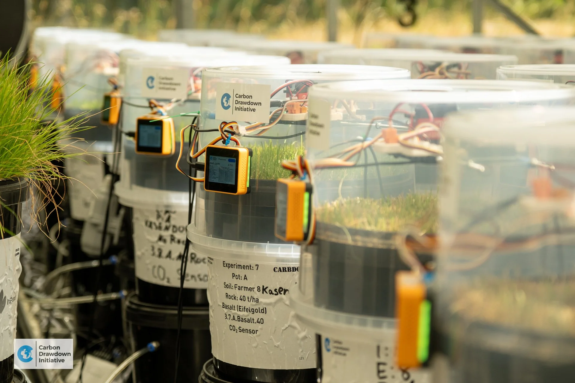
Our contribution to EW research is the creation of numerous datasets through our extensive greenhouse experiment where we have almost 400 lysimeter pots which contain combinations from 18 soils and 14 amendments.
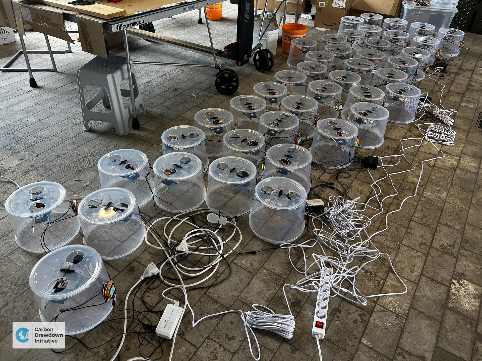
Besides the several measurement approaches that we are applying to observe the processes that go on in the soil of each lysimeter, we also want to measure the CO₂ efflux that comes out of the soil. This turns out to be no simple task as standard equipment can not do the job. So we had to build our own little army of 50 robotic fluxmeters that autonomously measure soil CO₂ effluxes every 10 minutes 24/7. This was possible at a surprisingly low price (compared to scientific instruments normally used for such measurements) of € 170 per device as we used low-cost standard electronics parts and low-cost plastic buckets as housings.
During calibration we found that in our specific greenhouse setup the accuracy of our self-made instruments is plus/minus 15% or better compared to a high-end scientific off-the-shelf soil CO₂ fluxmeter (LI-COR LI-870SC CO₂ Survey Soil Flux Package). An important achievement as 15% is much lower than most efflux changes we observed after the rock amendment.

Why not buy off-the-shelf flux meters?
Our greenhouse has almost 400 pots, a huge number that makes it not feasible to carry out manual CO₂ efflux measurements. At this scale we need an automated solution to do these measurements, especially when short intervals between 10 and 60 minutes and around-the-clock measurements are desired. Off-the-shelf flux meters (semi automated or carry-around) generally used for such scientific work are not suitable for us, as we would need a lot of people handling these in the greenhouse 24/7. They are also quite expensive (several 10,000 US$ per piece) and data handling requires a lot of manual work, file copying, etc. In short: It’s too expensive, too tedious, hardly scalable and quite error-prone for a project at our scale.
Our preliminary measurements with CO₂ sensors in the soils have shown that there are huge intra-day, day-to-day, week-to-week and seasonal variations in the soil CO₂ concentrations that drive the efflux (Fick's 1st law). This means that we must always measure controls and their respective treatments at the same time (night time is particularly important), otherwise we cannot directly compare control and treatment data. We also need continuous measurements throughout the season.
So we need a CO₂ efflux monitoring system that
consists of 50 individual fluxmeters that do not break our budget and that can be built quickly.
runs autonomously without requiring people on-site all the time (besides being expensive, increased ambient CO₂ levels from people handling the fluxmeters can increase signal noise levels as the relative CO₂ change in the chamber becomes smaller).
takes parallel measurements for many variations at the same time every 10 minutes.
works autonomously and stable 24/7.
stores data in a structured manner (what data point belongs to which pot experiment?) without error prone manual intervention.
provides automated data analysis for live data and alarms as well as long term analysis.
measures CO₂ concentration, barometric pressure, temperature, humidity and light inside each individual chamber.
controls an air fan for chamber air mixing and chamber flushing.
opens and closes the chamber using a servo motor.
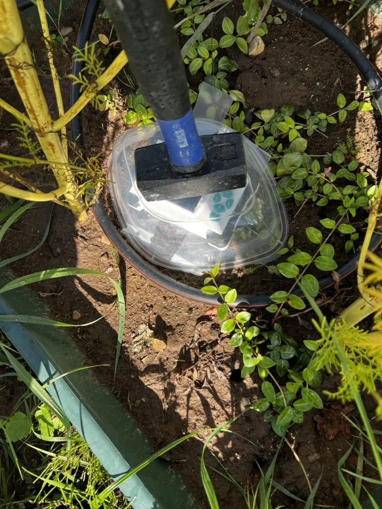
has a translucent chamber so the plants won’t die due to lack of light when the flux meter chambers sit on the lysimeters for a few days.
has a centralized control system and a method to update the software for all systems at once.
connects to the cloud for data storage, analysis, processing and monitoring.
As we did not find such a system, we decided to build our own. During this process, the specific circumstances of our project allowed us to dramatically simplify the concept of such fluxmeters. For example, the fact that we only use our fluxmeters on a specific pot size and in a greenhouse where there is no wind drastically simplified the sealing of the chamber. And since our devices are not moved around a lot, or exposed to the elements, we could make them out of cheap plastic and without the need for weatherproofing.
We went through 4 prototypes
On the way to the current CO₂ efflux meter design we went through four experimental prototypes (from left to right):


Prototype #1 (Sep 2022): We simply put a CO₂ sensor in a bucket that we placed onto our XXL lysimeters and watched the change in CO₂ concentration. We used an off-the-shelf CO₂ sensor with 1-min-interval data recording (€ 75, from Amazon) and obtained a vague signal of differences in CO₂ efflux between control and treatments.
Prototype #2 (Oct 2022): We completely sealed off the top of our XXL lysimeters and later of our pots in the greenhouse with a lid (manually) for 10 minutes and placed LoRaWAN CO₂ sensors beneath. Again, we saw a small difference in CO₂ efflux between controls and treatments.
Prototype #3 (Feb 2023): Using a robotics set from LEGO Mindstorms and plastic buckets we created a robotic fluxmeter that opened/closed the lid periodically and vented the chamber while we monitored the CO₂ concentration every minute using LoRaWAN CO₂ sensors. Worked, again.
Prototype #4 (May 2023): We build 8 fluxmeters using an ESP 32 microcontroller, a servo motor and a Sensirion SCD30 CO₂ sensor. Data was collected in a 3 second interval and immediately sent to the cloud for live analysis, the chamber was closed for 3 minutes every 10 minutes. We ran these for 6 weeks on many different variations in our greenhouse and we could see proper flux signals in the CO₂ data.
Based on the experiences from these 4 prototypes and encouraged by the fact that we could measure CO₂ effluxes that seemed to make sense and that also correlated to the soil pCO₂ measurements we had, we moved on to build prototype number 5.
Introducing: Carbdown Fluxmeter Generation 5
Of course we did not want to completely reinvent the wheel, so we looked for scientific publications on the topic. Where applicable, the basic setup and measurement process of our system is largely compliant with Maier et al. (2022) “Introduction of a guideline for measurements of greenhouse gas fluxes from soils using non-steady-state chambers” as well as Pavelka et al. (2018) Standardisation of chamber technique for CO₂, N2O and CH4 fluxes measurements from terrestrial ecosystems”.
The hardware of our current 5th generation CO₂ efflux meters is using a M5Stack Core 2 IoT controller in combination with the acclaimed Sensirion SCD30 CO₂ sensor which also gives us humidity and sensor-temperature data. We furthermore measure the light in the chamber (in the 400-700 nm spectrum of photosynthesis) to help us understand the photosynthesis effects during the day (M5Stack DLight sensor) as well as the barometric pressure and air temperature (M5Stack Barometric Pressure Unit sensor). This dataset enables us to calculate the actual CO₂ soil efflux whilst also taking into account the water vapor efflux.


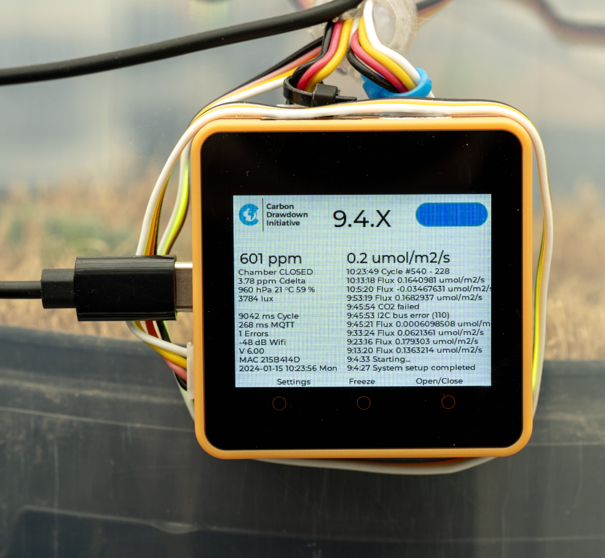
The tiny computers run our own firmware software (currently version 6) and control small 50x50 mm ventilators which are placed inside the chamber and have two jobs:
Quickly flushing out the chamber air at full fan speed when we open it after 3 minutes
Constantly moving ambient air into the chamber while the chamber is open
Gently mixing the air inside the chamber when the chamber is closed
Click to zoom in
When we are not flushing the chamber at full ventilator speed we intermittently power the ventilator on/off for 500 ms every few seconds so it does not get to nominal speed but instead creates a very gentle airflow. We tried various settings and eventually opted for the lowest flow that still shows a decently fast CO₂ signal increase after closing the chamber.
For the fluxmeter housing we use a transparent bucket with an opening slightly larger in diameter than the soil pots (both from the same supplier). Placement of this transparent bucket on top of the lysimeter pots creates a good seal because the diameter of the bottom of these buckets is smaller than the diameter of their top - and of the lysimeter pots.
The Hardware
Here is a list of all components along with a cost overview per fluxmeter (ca. € 170 in total per device).
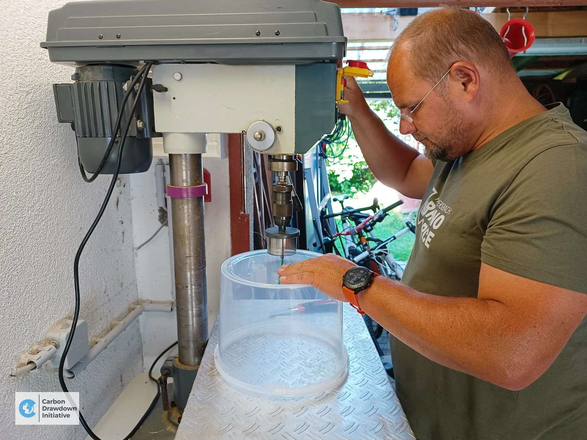
The Build process
Development, prototyping and also the building process took place in our CEO’s and CTO’s garages. Here are a few impressions (click the photos to zoom in):


The Controller Software


Our goal was to iterate quickly so we used a rapid-development approach. M5Stack, the vendor of the microcontrollers, offers a rapid-prototyping environment called UIFlow where we could write/change the software (visual programming using Blockly). It’s a “no-code” development environment. The photos what the controller’s user interface and the code in the visual programming environment look like:
The resulting Micropython code (ca. 1,200 lines of Python code) is then transferred to the controller via WiFi.
We installed our own small and simple bootloader software on each controller, which downloads the latest version of the actual flux meter controller code from the cloud every time the system is booted. This allows us to roll out new versions quickly by simply rebooting all the controllers remotely after uploading a new version.
Over time we implemented various tweaks to increase system stability and robustness so we avoid the need to drive to the greenhouse often to fix problems (e.g. automated hard reboots every 6 hours as a means of self-healing). We can also control all the fluxmeters by sending commands via MQTT (e.g. for synchronized sensor calibration, reboots or servo motor tests). Each fluxmeter is completely independent from the others, so if one breaks down the rest of them continue to carry out measurements.
When a fluxmeter is placed on a specific pot/experiment in the greenhouse the location code of the pot (“table.variant.replica”, e.g. 9.2.B) is entered into each controller via the touch screen. As soon as the measurements begin the computer synchronizes its clock via Internet and NTP protocol and then all data points are stored live, fully labeled and timestamped in the cloud-based time series database. This avoids error-prone manual intervention and data transfers. The live transfer of the data enables us to see results instantaneously (just seconds after measurement) on a Grafana dashboard. We also get instant hints on when a particular fluxmeter has a problem. The data pipeline is explained in the blog post How We Juggle Over 4 Million Data Points Daily in Real-Time.
The key element: The Sensirion SCD30 CO₂ sensor
The most important element in the fluxmeter is the CO₂ sensor. We are using the Sensirion SCD30 sensor (price ca. 55 €) with a nominal measurement range of 0 to 40,000 ppm and an advertised accuracy of ± (30 ppm plus 3 % of the measurement value). The Sensirion SCD30 sensor module is a dual channel NDIR CO₂ sensor which means it can be used over a long time without recalibration. It has a second chamber filled with a gas that is stable since its manufacture, does not change and whose infrared absorption properties are well known. By analyzing the subtle differences in the measurement results of that gas in chamber 2, the sensor firmware can calculate how much the measurements have deviated from what they should be and can apply a correction to the gas concentration measured in chamber 1.
The vendor’s CO₂ sensor specifications (link) are:
Overall CO₂ measurement range: 0 – 40,000 ppm
Accuracy between 400 ppm and 10,000 ppm: ± (30 ppm + 3%)
Repeatability between 400 ppm and 10,000 ppm: ± 10 ppm
Temperature stability between 0° C and 50° C: ± 2.5 ppm / °C
Humidity: Measurement range (25°C) 0 – 100 % RH with ± 3 % RH accuracy
Temperature: Measurement range 0° C – 50° C with ± (0.4° C + 0.023 × (T [° C] – 25° C)) accuracy
The SCD30 sensor was already reviewed in two scientific studies: “Therefore only the K30 FR (and to a much lower extent the SCD30) with its fast response time and high response strength passed laboratory validation and met all necessary requirements for accurate and precise in situ measurements of CO₂ exchange.” (Macagga et al. 2023, preprint). They continue: “Also findings of González Rivero et al. (2023), who tested the ability of the SCD30 to reflect calibration gas concentrations and concluded an acceptable accuracy and response time, are in a good agreement with results of the present study.” In both studies, the SCD30 sensor is reported to slightly overestimate the increase of the CO₂ concentration. However, during calibration tests we did not find any problems that might be caused by this.
Potential inaccuracies
One potentially major source of inaccuracy in our system is the volume of the chamber because:
In some pots the soil has settled more than in others (vertical height of the soil column can differ by up to 1-2 cm which with a chamber height of 16-17 cm results in a potential error of up to 6-12%). This issue mostly depends on the soil type which is the same for simultaneously measured treatments and their respective controls. So when we subtract the CO₂ efflux of the control from the treatment to get the difference in efflux, this error mostly cancels out.
The amount of plant biomass (and with it, plant volume) also differs between pots. This effect is often the same for replicas of one variation, but different between variations (e.g. by varying fertilizer effects of the rocks). We try to minimize this effect by cutting the grass every time before we install the flux meters. This way, any error introduced by the volume difference in biomass should be quite small.
In contrast to most industrial flux meters our chamber is transparent which means that in daylight the photosynthesis of the plants remains active during chamber-closed-phases. Depending on the amount of biomass and light this reduces the CO₂ concentration quite quickly and skews the daytime flux measurements (on sunny days we sometimes see how the CO₂ concentration in the chamber drops from e.g. 600 ppm to 400 ppm in less than three minutes as soon as the chamber is closed, nature’s photosynthesis CO₂ capturing power at work).
When we calibrated our fluxmeters against a high-end professional fluxmeter we found that our nighttime data (=in darkness) was the best fit. So for the data analysis we filter the data and only use the data points with a lightmeter-reading of 10 lux or less. Cueva et al. (2017) also found night data to be most suitable for what we want to do: “We propose a simple method, based on the temporal stability concept, to determine the most appropriate time of the day for manual measurements to capture a representative mean daily Rs value. (..) In general, we found optimum times were at night.”
A technical problem that we improved over time was what we call “stuck chambers” which occurred when the servo motor sometimes failed to open/close the chamber properly. The chamber was then stuck in an open or closed state for hours up to days until we could fix it manually. A small change in the software improved this: By exercising the movement, i.e. rotating twice through the whole 270° range of the servo in every cycle (instead of only going back and forth by 90°) this problem was solved almost completely. To avoid that a rare occurrence of “stuck chambers” potentially distorts our efflux data we remove all fluxes below 0.1 µmol/m²/s during the data analysis. Effectively all remaining valid data points were above this value after removing all data above 10 lux in the previous step anyway.
Another problem that renders very similar efflux data is what we call “clogged pots”. We saw hours and even days of close to zero fluxes on some pots despite the servo working fine all the time. In some of these cases the pots also had pCO₂ sensors in the soil and showed very high CO₂ levels (>20.000 ppm). Apparently the gasses couldn’t get out, not even the air humidity changed during chamber cycles. As this happened more often during the summer when we had to increase irrigation, we think this is a greenhouse/experiment-specific issue with excess water blocking the gas flow in the soil. These failed measurements are also removed by the filtering described above for the stuck chambers.

Hourly measurements of the fluxmeters for 7.1, denoted by their MAC addresses
Here is an extreme example of clogged pots/stuck chambers: variant 7.1 had one or two zero-flux pots from August to October (blue arrows, non-linear x-axis, i.e. time spans without data are not shown, numbers are month/day/hour).

Our filtering approach led to the removal of 20%-40% of the data in that time (graph shows % rate of filtered data per week, again time spans without data are not shown):

When the data of the replicas is averaged over the available time the average changes from 0.56 µmol/m²/s (unfiltered, left) to the much more correct value of 0.78 µmol/m²/s (filtered, right).
In an attempt to distinguish better between the low fluxes which increasingly showed up while we went into fall (seasonal effects due to less biological activity and light), and stuck chambers or clogged pots, we implemented a dynamic chamber cycle time in version 6 of the firmware (October 2023). The normal chamber cycle is 3 minutes. If the change of CO₂ concentration in the chamber is still below 5 ppm 3 minutes after closing the chamber the chamber is kept closed for up to 2 more minutes or until the change is higher, whatever comes first. We effectively give the CO₂ gas 66% more time to increase during low flux-season which improves the measurements.
The following graph shows the effect of the firmware change for all flux measurements (colors show table numbers, x-axis is time in month-day-hour): During the first weeks the clogged/stuck issues increased and during September and October we need to filter 5-20% of the data, depending on the table number (= soil type). 25% filter rate would mean that we have reduced the number of replicas per variant from 4 to 3.

After October 22nd the filter rate dropped considerably with the new firmware, only increasing again during December when the actual efflux rates become quite low due to the seasonal circumstances and the data distortion potential is very low:
Other potential inaccuracies
Other inaccuracies that can come from the various other sensors are as follows (vendor data):
Pressure sensor (link):
Barometric pressure: Measurement range 30 kPa to 110 kPa with ±3.9 kPa accuracy
Temperature: Measurement range -20°C to 65°C with ± 2 °C accuracy.
Light sensor (link):
Measurement range 0 lux to 65.000 lux (based on photosynthesis relevant spectrum of 400-700 nm) with ±1.2% accuracy.
For chamber air temperature we use the pressure sensor’s data because the CO₂ sensor heats up during constant measurement and is constantly 1-2°C warmer than the air.
All time related metrics of the flux calculations are measured in ms (1/1000 s) by the controller, so timing inaccuracies should not be of any concern.
Propagating all these potential inaccuracies we expected an accuracy of the flux measurements between ±10-15% for most measurements, which upon calibration turned out to be a good estimate.
Sensor Calibration and Noise Levels
To assess the differences between the efflux of a treated and untreated control we need to perform two steps:
First we subtract two measurements of one sensor per fluxmeter (at beginning and end of the chamber cycle, simplified) to get the change in CO₂ concentration during the chamber cycle.
Then we subtract two of these flux measurements (control vs. treatment) from each other to understand the effects of the treatment on CO₂ fluxes.
This means that relative inaccuracies between a lower and a higher measurement taken by one individual sensor are more relevant than the absolute accuracy of the sensors between each other.
To investigate and mitigate these effects, we calibrated the sensors to the same CO₂ levels and then observed how different the measurements were afterwards.

When we put the first 50 sensors into a room on the floor, flushed the air by opening the large, floor-level window for 1 hour, and then sent the calibration command (sets all sensors to 420 ppm), we got this result.
The factory calibration is obviously not good, the sensor should not be used without calibration. But after calibration the sensor measurements stay close to each other.

When we had built all 85 sensors, we did the same thing again, tracking the minute-by-minute measurements for 15 hours.
The black lines show minimum, average and maximum. The red line (uses the right axis) shows the standard deviations in ppm for every minute for 85 sensors. This value remains between 14 and 17 ppm (=3-4%) all the time, which is better than the advertised accuracy between 400 ppm and 10,000 ppm of ± (30 ppm + 3%).

We then used CO₂ from a household CO₂ cartridge to raise the room's CO₂ concentration to 1,800 ppm and then to 2,100 ppm, and followed the measurements for 18 hours, when the room's CO₂ concentration finally returned to 480 ppm. The graph shows only the first hour, the black line shows the average concentration, red is the standard deviation which naturally goes up while the CO₂ gas is spread in the room and reaches the sensors one by one. It is interesting that it took the CO₂ only about 5 minutes to disperse evenly.

When we plot the observed standard deviations against the CO₂ concentration, we see that the relative standard deviations decrease from 4.8% at 500 ppm to 2.3% at 1,800 ppm. Lower deviations with higher concentrations are particularly good for soil pCO₂ sensors which usually see very high ppm numbers. For fluxmeters the range between 500-600 ppm up to 1,000 ppm is important where we see around 4% deviation.
How accurate are the robot army fluxmeters in practice?

During our calibration tests we found that the full inaccuracy of our measurements are mostly in the order of up to 15% (when comparing one hour averages of 4 replicas) compared to a high-end off-the-shelf device, often even better. We used the LI-COR LI-870SC CO₂ Survey Soil Flux Package, i.e. the LI-870 CO₂/H₂O Gas Analyzer with the 8200-01S Smart Chamber, details in an upcoming paper.

This graph shows the measurements of the reference off-the-shelf fluxmeter and our fluxmeter army. In an ideal world the dots and boxes of both series would be located on the diagonal. Most of the fluxmeter army measurements are in a band of ± 15% of the reference fluxmeter’s measurements.
Given the fact that the soil heterogeneity together with the amendment-induced differences in the effluxes are clearly larger than that (we found that the treatment efflux can be 20-60% higher than the efflux from its respective control) we think we have built a pretty good foundation for scientifically sound CO₂ efflux measurements in the context of ERW in a greenhouse experiment. Especially when we take into account that without the fluxmeter army we would not be able to get the necessary amount and frequency of data at all.
Proofing Fick’s 1st Law

Relationship between delta of ambient CO₂ and average soil pCO₂ in 2023 and CO₂ efflux (Jul-Dec 2023) for experiments on tables 5, 6, 7 and 9.
According to Fick’s 1st law there should be a linear relationship between the pCO₂ concentration in the soil gas and the resulting CO₂ efflux. We have 200 soil pCO₂ sensors built into selected pots from our greenhouse experiment. The following graphs show this relationship, which is another way of truthing our flux measurements. The different gradients of the positive correlations for each table reflects the different diffusion factors that depend on soil specific parameters; each of the four tables uses a different soil.
These plots suggest that it may be sufficient to monitor fluxes using the much cheaper and less complex pCO₂ sensors during periods when fluxmeter data are not available.
Moving the army into the greenhouse and getting started
Here is a short video that shows how we transported the finished fluxmeters to the greenhouse and installed them for the first time.
Daily and weekly maintenance
Once or twice per week we groom the grass on the next table and then move the fluxmeters over. This can be seen in this timelapse.
Next step: Looking at the actual data
To get an insight into the first data that resulted from 7 months of measurements with our fluxmeter army we refer you to our article about our CO₂ efflux measurements results due to be published shortly.
References
If you want to read more about CO₂ fluxmeters, here are a few documents that we found helpful:
Licor Inc., Support document Soil gas flux measurement theory https://www.licor.com/env/support/Smart-Chamber/topics/the-measurement-cycle.html
Gasmet Technologies Oy, White paper “Greenhouse Gas Flux Measurements”
Maier et al., 2022, Introduction of a guideline for measurements of greenhouse gas fluxes from soils using non-steady-state chambers
Pavelka et al., 2018, Standardisation of chamber technique for CO₂, N2O and CH4 fluxes measurements from terrestrial ecosystems
Zhao et al., 2018, On the calculation of daytime CO₂ fluxes measured by automated closed transparent chambers
Pirk at al., 2016, Calculations of automatic chamber flux measurements of methane and carbon dioxide using short time series of concentrations
Macagga et al., 2023, Validation and field application of a low-cost device to measure CO2 and ET fluxes (preprint)
Cueva at al., 2017, Potential bias of daily soil CO2 efflux estimates due to sampling time
Paessler et al., 2023, 24/7 Monitoring of soil gas pCO₂ concentrations in large scale ERW experiments with low cost electronics